10分钟入门pandas
INFO
原文为 10 minutes to pandas。对应版本 2.3(stable)。 由 Gemini 2.5 Pro 翻译,请对内容进行甄别。
这是一篇pandas的简短介绍,主要面向新用户。你可以在Cookbook中看到更复杂的诀窍。
按照惯例,我们如下导入:
In [1]: import numpy as np

In [2]: import pandas as pdpandas中的基本数据结构
Pandas提供了两种用于处理数据的类:
对象创建
请参阅数据结构介绍部分。
通过传递一个值列表来创建一个Series,让pandas创建一个默认的RangeIndex。
In [3]: s = pd.Series([1, 3, 5, np.nan, 6, 8])

In [4]: s
Out[4]:
0    1.0
1    3.0
2    5.0
3    NaN
4    6.0
5    8.0
dtype: float64通过传递一个带有日期时间索引(使用date_range())和带标签的列的NumPy数组来创建一个DataFrame:
In [5]: dates = pd.date_range("20130101", periods=6)

In [6]: dates
Out[6]:
DatetimeIndex(['2013-01-01', '2013-01-02', '2013-01-03', '2013-01-04',
               '2013-01-05', '2013-01-06'],
              dtype='datetime64[ns]', freq='D')

In [7]: df = pd.DataFrame(np.random.randn(6, 4), index=dates, columns=list("ABCD"))

In [8]: df
Out[8]:
                   A         B         C         D
2013-01-01  0.469112 -0.282863 -1.509059 -1.135632
2013-01-02  1.212112 -0.173215  0.119209 -1.044236
2013-01-03 -0.861849 -2.104569 -0.494929  1.071804
2013-01-04  0.721555 -0.706771 -1.039575  0.271860
2013-01-05 -0.424972  0.567020  0.276232 -1.087401
2013-01-06 -0.673690 0.113648 -1.478427 0.524988通过传递一个字典对象来创建一个DataFrame,其中键是列标签,值是列的值。
In [9]: df2 = pd.DataFrame(
   ...:     {
   ...:         "A": 1.0,
   ...:         "B": pd.Timestamp("20130102"),
   ...:         "C": pd.Series(1, index=list(range(4)), dtype="float32"),
   ...:         "D": np.array([3] * 4, dtype="int32"),
   ...:         "E": pd.Categorical(["test", "train", "test", "train"]),
   ...:         "F": "foo",
   ...:     }
   ...: )
   ...:

In [10]: df2
Out[10]:
     A          B    C  D      E    F
0  1.0 2013-01-02  1.0  3   test  foo
1  1.0 2013-01-02  1.0  3  train  foo
2  1.0 2013-01-02  1.0  3   test  foo
3 1.0 2013-01-02 1.0 3 train fooIn [11]: df2.dtypes
Out[11]:
A float64
B datetime64[ns]
C float32
D int32
E category
F object
dtype: object如果你正在使用IPython,列名(以及公共属性)的制表符补全功能是自动启用的。以下是将被补全的属性的一个子集:
In [12]: df2.<TAB>  # noqa: E225, E999
df2.A                  df2.bool
df2.abs                df2.boxplot
df2.add                df2.C
df2.add_prefix         df2.clip
df2.add_suffix         df2.columns
df2.align              df2.copy
df2.all                df2.count
df2.any                df2.combine
df2.append             df2.D
df2.apply              df2.describe
df2.applymap           df2.diff
df2.B df2.duplicated如你所见,列A、B、C和D会自动进行制表符补全。E和F也在那里;为了简洁,其余的属性已被截断。
查看数据
请参阅基础功能部分。
分别使用DataFrame.head()和DataFrame.tail()来查看数据框的头部和尾部行:
In [13]: df.head()
Out[13]:
                   A         B         C         D
2013-01-01  0.469112 -0.282863 -1.509059 -1.135632
2013-01-02  1.212112 -0.173215  0.119209 -1.044236
2013-01-03 -0.861849 -2.104569 -0.494929  1.071804
2013-01-04  0.721555 -0.706771 -1.039575  0.271860
2013-01-05 -0.424972  0.567020  0.276232 -1.087401

In [14]: df.tail(3)
Out[14]:
                   A         B         C         D
2013-01-04  0.721555 -0.706771 -1.039575  0.271860
2013-01-05 -0.424972  0.567020  0.276232 -1.087401
2013-01-06 -0.673690 0.113648 -1.478427 0.524988显示DataFrame.index或DataFrame.columns:
In [15]: df.index
Out[15]:
DatetimeIndex(['2013-01-01', '2013-01-02', '2013-01-03', '2013-01-04',
               '2013-01-05', '2013-01-06'],
              dtype='datetime64[ns]', freq='D')

In [16]: df.columns
Out[16]: Index(['A', 'B', 'C', 'D'], dtype='object')使用DataFrame.to_numpy()返回底层数据的NumPy表示,不包括索引或列标签:
In [17]: df.to_numpy()
Out[17]:
array([[ 0.4691, -0.2829, -1.5091, -1.1356],
       [ 1.2121, -0.1732,  0.1192, -1.0442],
       [-0.8618, -2.1046, -0.4949,  1.0718],
       [ 0.7216, -0.7068, -1.0396,  0.2719],
       [-0.425 ,  0.567 ,  0.2762, -1.0874],
[-0.6737, 0.1136, -1.4784, 0.525 ]])WARNING
NumPy数组对于整个数组只有一个dtype,而pandas DataFrame每列有一个dtype。当你调用DataFrame.to_numpy()时,pandas会找到可以容纳DataFrame中所有dtypes的NumPy dtype。如果公共数据类型是object,DataFrame.to_numpy()将需要复制数据。
In [18]: df2.dtypes
Out[18]:
A                 float64
B          datetime64[ns]
C                 float32
D                   int32
E                category
F                  object
dtype: object

In [19]: df2.to_numpy()
Out[19]:
array([[1.0, Timestamp('2013-01-02 00:00:00'), 1.0, 3, 'test', 'foo'],
       [1.0, Timestamp('2013-01-02 00:00:00'), 1.0, 3, 'train', 'foo'],
       [1.0, Timestamp('2013-01-02 00:00:00'), 1.0, 3, 'test', 'foo'],
       [1.0, Timestamp('2013-01-02 00:00:00'), 1.0, 3, 'train', 'foo']],
dtype=object)describe()显示了数据的快速统计摘要:
In [20]: df.describe()
Out[20]:
              A         B         C         D
count  6.000000  6.000000  6.000000  6.000000
mean   0.073711 -0.431125 -0.687758 -0.233103
std    0.843157  0.922818  0.779887  0.973118
min   -0.861849 -2.104569 -1.509059 -1.135632
25%   -0.611510 -0.600794 -1.368714 -1.076610
50%    0.022070 -0.228039 -0.767252 -0.386188
75%    0.658444  0.041933 -0.034326  0.461706
max 1.212112 0.567020 0.276232 1.071804转置数据:
In [21]: df.T
Out[21]:
   2013-01-01  2013-01-02  2013-01-03  2013-01-04  2013-01-05  2013-01-06
A    0.469112    1.212112   -0.861849    0.721555   -0.424972   -0.673690
B   -0.282863   -0.173215   -2.104569   -0.706771    0.567020    0.113648
C   -1.509059    0.119209   -0.494929   -1.039575    0.276232   -1.478427
D -1.135632 -1.044236 1.071804 0.271860 -1.087401 0.524988In [22]: df.sort_index(axis=1, ascending=False)
Out[22]:
D C B A
2013-01-01 -1.135632 -1.509059 -0.282863 0.469112
2013-01-02 -1.044236 0.119209 -0.173215 1.212112
2013-01-03 1.071804 -0.494929 -2.104569 -0.861849
2013-01-04 0.271860 -1.039575 -0.706771 0.721555
2013-01-05 -1.087401 0.276232 0.567020 -0.424972
2013-01-06 0.524988 -1.478427 0.113648 -0.673690In [23]: df.sort_values(by="B")
Out[23]:
A B C D
2013-01-03 -0.861849 -2.104569 -0.494929 1.071804
2013-01-04 0.721555 -0.706771 -1.039575 0.271860
2013-01-01 0.469112 -0.282863 -1.509059 -1.135632
2013-01-02 1.212112 -0.173215 0.119209 -1.044236
2013-01-06 -0.673690 0.113648 -1.478427 0.524988
2013-01-05 -0.424972 0.567020 0.276232 -1.087401选择
WARNING
虽然标准的Python / NumPy选择和设置表达式很直观,并且在交互式工作中很方便,但对于生产代码,我们建议使用优化的pandas数据访问方法:DataFrame.at()、DataFrame.iat()、DataFrame.loc()和DataFrame.iloc()。
Getitem ([])
对于DataFrame,传递单个标签会选择一列,并产生一个等同于df.A的Series:
In [24]: df["A"]
Out[24]:
2013-01-01    0.469112
2013-01-02    1.212112
2013-01-03   -0.861849
2013-01-04    0.721555
2013-01-05   -0.424972
2013-01-06   -0.673690
Freq: D, Name: A, dtype: float64对于DataFrame,传递一个切片:会选择匹配的行:
In [25]: df[0:3]
Out[25]:
                   A         B         C         D
2013-01-01  0.469112 -0.282863 -1.509059 -1.135632
2013-01-02  1.212112 -0.173215  0.119209 -1.044236
2013-01-03 -0.861849 -2.104569 -0.494929  1.071804

In [26]: df["20130102":"20130104"]
Out[26]:
                   A         B         C         D
2013-01-02  1.212112 -0.173215  0.119209 -1.044236
2013-01-03 -0.861849 -2.104569 -0.494929  1.071804
2013-01-04 0.721555 -0.706771 -1.039575 0.271860按标签选择
请参阅按标签选择中使用DataFrame.loc()或DataFrame.at()的更多信息。
选择与标签匹配的行:
In [27]: df.loc[dates[0]]
Out[27]:
A    0.469112
B   -0.282863
C   -1.509059
D   -1.135632
Name: 2013-01-01 00:00:00, dtype: float64选择所有行(:)和指定的列标签:
In [28]: df.loc[:, ["A", "B"]]
Out[28]:
                   A         B
2013-01-01  0.469112 -0.282863
2013-01-02  1.212112 -0.173215
2013-01-03 -0.861849 -2.104569
2013-01-04  0.721555 -0.706771
2013-01-05 -0.424972  0.567020
2013-01-06 -0.673690 0.113648对于标签切片,两个端点都包含在内:
In [29]: df.loc["20130102":"20130104", ["A", "B"]]
Out[29]:
                   A         B
2013-01-02  1.212112 -0.173215
2013-01-03 -0.861849 -2.104569
2013-01-04 0.721555 -0.706771选择单个行和列标签会返回一个标量:
In [30]: df.loc[dates[0], "A"]
Out[30]: 0.4691122999071863为了快速访问一个标量(等同于前一个方法):
In [31]: df.at[dates[0], "A"]
Out[31]: 0.4691122999071863按位置选择
请参阅按位置选择中使用DataFrame.iloc()或DataFrame.iat()的更多信息。
通过传递的整数位置进行选择:
In [32]: df.iloc[3]
Out[32]:
A    0.721555
B   -0.706771
C   -1.039575
D    0.271860
Name: 2013-01-04 00:00:00, dtype: float64整数切片的作用类似于NumPy/Python:
In [33]: df.iloc[3:5, 0:2]
Out[33]:
                   A         B
2013-01-04  0.721555 -0.706771
2013-01-05 -0.424972 0.567020整数位置位置列表:
In [34]: df.iloc[[1, 2, 4], [0, 2]]
Out[34]:
                   A         C
2013-01-02  1.212112  0.119209
2013-01-03 -0.861849 -0.494929
2013-01-05 -0.424972 0.276232要显式地对行进行切片:
In [35]: df.iloc[1:3, :]
Out[35]:
                   A         B         C         D
2013-01-02  1.212112 -0.173215  0.119209 -1.044236
2013-01-03 -0.861849 -2.104569 -0.494929 1.071804要显式地对列进行切片:
In [36]: df.iloc[:, 1:3]
Out[36]:
                   B         C
2013-01-01 -0.282863 -1.509059
2013-01-02 -0.173215  0.119209
2013-01-03 -2.104569 -0.494929
2013-01-04 -0.706771 -1.039575
2013-01-05  0.567020  0.276232
2013-01-06 0.113648 -1.478427要显式地获取一个值:
In [37]: df.iloc[1, 1]
Out[37]: -0.17321464905330858为了快速访问一个标量(等同于前一个方法):
In [38]: df.iat[1, 1]
Out[38]: -0.17321464905330858布尔索引
选择df.A大于0的行。
In [39]: df[df["A"] > 0]
Out[39]:
                   A         B         C         D
2013-01-01  0.469112 -0.282863 -1.509059 -1.135632
2013-01-02  1.212112 -0.173215  0.119209 -1.044236
2013-01-04 0.721555 -0.706771 -1.039575 0.271860从DataFrame中选择满足布尔条件的值:
In [40]: df[df > 0]
Out[40]:
                   A         B         C         D
2013-01-01  0.469112       NaN       NaN       NaN
2013-01-02  1.212112       NaN  0.119209       NaN
2013-01-03       NaN       NaN       NaN  1.071804
2013-01-04  0.721555       NaN       NaN  0.271860
2013-01-05       NaN  0.567020  0.276232       NaN
2013-01-06 NaN 0.113648 NaN 0.524988使用isin()方法进行过滤:
In [41]: df2 = df.copy()

In [42]: df2["E"] = ["one", "one", "two", "three", "four", "three"]

In [43]: df2
Out[43]:
                   A         B         C         D      E
2013-01-01  0.469112 -0.282863 -1.509059 -1.135632    one
2013-01-02  1.212112 -0.173215  0.119209 -1.044236    one
2013-01-03 -0.861849 -2.104569 -0.494929  1.071804    two
2013-01-04  0.721555 -0.706771 -1.039575  0.271860  three
2013-01-05 -0.424972  0.567020  0.276232 -1.087401   four
2013-01-06 -0.673690  0.113648 -1.478427  0.524988  three

In [44]: df2[df2["E"].isin(["two", "four"])]
Out[44]:
                   A         B         C         D     E
2013-01-03 -0.861849 -2.104569 -0.494929  1.071804   two
2013-01-05 -0.424972 0.567020 0.276232 -1.087401 four设置
设置一个新列会根据索引自动对齐数据:
In [45]: s1 = pd.Series([1, 2, 3, 4, 5, 6], index=pd.date_range("20130102", periods=6))

In [46]: s1
Out[46]:
2013-01-02    1
2013-01-03    2
2013-01-04    3
2013-01-05    4
2013-01-06    5
2013-01-07    6
Freq: D, dtype: int64

In [47]: df["F"] = s1按标签设置值:
In [48]: df.at[dates[0], "A"] = 0按位置设置值:
In [49]: df.iat[0, 1] = 0通过使用NumPy数组赋值进行设置:
In [50]: df.loc[:, "D"] = np.array([5] * len(df))前面设置操作的结果:
In [51]: df
Out[51]:
                   A         B         C    D    F
2013-01-01  0.000000  0.000000 -1.509059  5.0  NaN
2013-01-02  1.212112 -0.173215  0.119209  5.0  1.0
2013-01-03 -0.861849 -2.104569 -0.494929  5.0  2.0
2013-01-04  0.721555 -0.706771 -1.039575  5.0  3.0
2013-01-05 -0.424972  0.567020  0.276232  5.0  4.0
2013-01-06 -0.673690 0.113648 -1.478427 5.0 5.0带设置的where操作:
In [52]: df2 = df.copy()

In [53]: df2[df2 > 0] = -df2

In [54]: df2
Out[54]:
                   A         B         C    D    F
2013-01-01  0.000000  0.000000 -1.509059 -5.0  NaN
2013-01-02 -1.212112 -0.173215 -0.119209 -5.0 -1.0
2013-01-03 -0.861849 -2.104569 -0.494929 -5.0 -2.0
2013-01-04 -0.721555 -0.706771 -1.039575 -5.0 -3.0
2013-01-05 -0.424972 -0.567020 -0.276232 -5.0 -4.0
2013-01-06 -0.673690 -0.113648 -1.478427 -5.0 -5.0缺失数据
对于NumPy数据类型,np.nan表示缺失数据。默认情况下,它不包含在计算中。请参阅缺失数据部分。
重新索引允许您更改/添加/删除指定轴上的索引。这将返回数据的副本:
In [55]: df1 = df.reindex(index=dates[0:4], columns=list(df.columns) + ["E"])

In [56]: df1.loc[dates[0] : dates[1], "E"] = 1

In [57]: df1
Out[57]:
                   A         B         C    D    F    E
2013-01-01  0.000000  0.000000 -1.509059  5.0  NaN  1.0
2013-01-02  1.212112 -0.173215  0.119209  5.0  1.0  1.0
2013-01-03 -0.861849 -2.104569 -0.494929  5.0  2.0  NaN
2013-01-04 0.721555 -0.706771 -1.039575 5.0 3.0 NaNDataFrame.dropna()删除任何有缺失数据的行:
In [58]: df1.dropna(how="any")
Out[58]:
                   A         B         C    D    F    E
2013-01-02 1.212112 -0.173215 0.119209 5.0 1.0 1.0DataFrame.fillna()填充缺失数据:
In [59]: df1.fillna(value=5)
Out[59]:
                   A         B         C    D    F    E
2013-01-01  0.000000  0.000000 -1.509059  5.0  5.0  1.0
2013-01-02  1.212112 -0.173215  0.119209  5.0  1.0  1.0
2013-01-03 -0.861849 -2.104569 -0.494929  5.0  2.0  5.0
2013-01-04 0.721555 -0.706771 -1.039575 5.0 3.0 5.0isna()获取值为nan的布尔掩码:
In [60]: pd.isna(df1)
Out[60]:
                A      B      C      D      F      E
2013-01-01  False  False  False  False   True  False
2013-01-02  False  False  False  False  False  False
2013-01-03  False  False  False  False  False   True
2013-01-04 False False False False False True操作
请参阅关于二元操作的基础部分。
统计
通常,操作排除缺失数据。
计算每列的平均值:
In [61]: df.mean()
Out[61]:
A   -0.004474
B   -0.383981
C   -0.687758
D    5.000000
F    3.000000
dtype: float64计算每行的平均值:
In [62]: df.mean(axis=1)
Out[62]:
2013-01-01    0.872735
2013-01-02    1.431621
2013-01-03    0.707731
2013-01-04    1.395042
2013-01-05    1.883656
2013-01-06    1.592306
Freq: D, dtype: float64与具有不同索引或列的另一个Series或DataFrame进行操作将使结果与索引或列标签的并集对齐。此外,pandas会自动沿指定维度进行广播,并用np.nan填充未对齐的标签。
In [63]: s = pd.Series([1, 3, 5, np.nan, 6, 8], index=dates).shift(2)

In [64]: s
Out[64]:
2013-01-01    NaN
2013-01-02    NaN
2013-01-03    1.0
2013-01-04    3.0
2013-01-05    5.0
2013-01-06    NaN
Freq: D, dtype: float64

In [65]: df.sub(s, axis="index")
Out[65]:
                   A         B         C    D    F
2013-01-01       NaN       NaN       NaN  NaN  NaN
2013-01-02       NaN       NaN       NaN  NaN  NaN
2013-01-03 -1.861849 -3.104569 -1.494929  4.0  1.0
2013-01-04 -2.278445 -3.706771 -4.039575  2.0  0.0
2013-01-05 -5.424972 -4.432980 -4.723768  0.0 -1.0
2013-01-06 NaN NaN NaN NaN NaN用户定义函数
DataFrame.agg()和DataFrame.transform()分别应用用户定义的函数,该函数会减少或广播其结果。
In [66]: df.agg(lambda x: np.mean(x) * 5.6)
Out[66]:
A    -0.025054
B    -2.150294
C    -3.851445
D    28.000000
F    16.800000
dtype: float64

In [67]: df.transform(lambda x: x * 101.2)
Out[67]:
                     A           B           C      D      F
2013-01-01    0.000000    0.000000 -152.716721  506.0    NaN
2013-01-02  122.665737  -17.529322   12.063922  506.0  101.2
2013-01-03  -87.219115 -212.982405  -50.086843  506.0  202.4
2013-01-04   73.021382  -71.525239 -105.204988  506.0  303.6
2013-01-05  -43.007200   57.382459   27.954680  506.0  404.8
2013-01-06 -68.177398 11.501219 -149.616767 506.0 506.0值计数
请参阅直方图和离散化获取更多信息。
In [68]: s = pd.Series(np.random.randint(0, 7, size=10))

In [69]: s
Out[69]:
0    4
1    2
2    1
3    2
4    6
5    4
6    4
7    6
8    4
9    4
dtype: int64

In [70]: s.value_counts()
Out[70]:
4    5
2    2
6    2
1    1
Name: count, dtype: int64字符串方法
Series在str属性中配备了一套字符串处理方法,可以方便地对数组的每个元素进行操作,如下面的代码片段所示。请参阅矢量化字符串方法获取更多信息。
In [71]: s = pd.Series(["A", "B", "C", "Aaba", "Baca", np.nan, "CABA", "dog", "cat"])

In [72]: s.str.lower()
Out[72]:
0       a
1       b
2       c
3    aaba
4    baca
5     NaN
6    caba
7     dog
8     cat
dtype: object合并
Concat
pandas提供了各种便利的功能,可以轻松地将Series和DataFrame对象与各种集合逻辑结合起来,用于索引和关系代数功能,在连接/合并类型的操作中。
请参阅合并部分。
使用concat()按行连接pandas对象:
In [73]: df = pd.DataFrame(np.random.randn(10, 4))

In [74]: df
Out[74]:
          0         1         2         3
0 -0.548702  1.467327 -1.015962 -0.483075
1  1.637550 -1.217659 -0.291519 -1.745505
2 -0.263952  0.991460 -0.919069  0.266046
3 -0.709661  1.669052  1.037882 -1.705775
4 -0.919854 -0.042379  1.247642 -0.009920
5  0.290213  0.495767  0.362949  1.548106
6 -1.131345 -0.089329  0.337863 -0.945867
7 -0.932132  1.956030  0.017587 -0.016692
8 -0.575247  0.254161 -1.143704  0.215897
9  1.193555 -0.077118 -0.408530 -0.862495

# break it into pieces
In [75]: pieces = [df[:3], df[3:7], df[7:]]

In [76]: pd.concat(pieces)
Out[76]:
          0         1         2         3
0 -0.548702  1.467327 -1.015962 -0.483075
1  1.637550 -1.217659 -0.291519 -1.745505
2 -0.263952  0.991460 -0.919069  0.266046
3 -0.709661  1.669052  1.037882 -1.705775
4 -0.919854 -0.042379  1.247642 -0.009920
5  0.290213  0.495767  0.362949  1.548106
6 -1.131345 -0.089329  0.337863 -0.945867
7 -0.932132  1.956030  0.017587 -0.016692
8 -0.575247  0.254161 -1.143704  0.215897
9 1.193555 -0.077118 -0.408530 -0.862495WARNING
向DataFrame添加一列相对较快。但是,添加一行需要复制,并且可能很昂贵。我们建议将预先构建的记录列表传递给DataFrame构造函数,而不是通过迭代地向其附加记录来构建DataFrame。
Join
merge()可以实现沿特定列的SQL风格的连接类型。请参阅数据库风格的连接部分。
In [77]: left = pd.DataFrame({"key": ["foo", "foo"], "lval": [1, 2]})

In [78]: right = pd.DataFrame({"key": ["foo", "foo"], "rval": [4, 5]})

In [79]: left
Out[79]:
   key  lval
0  foo     1
1  foo     2

In [80]: right
Out[80]:
   key  rval
0  foo     4
1  foo     5

In [81]: pd.merge(left, right, on="key")
Out[81]:
   key  lval  rval
0  foo     1     4
1  foo     1     5
2  foo     2     4
3 foo 2 5在唯一键上使用merge():
In [82]: left = pd.DataFrame({"key": ["foo", "bar"], "lval": [1, 2]})

In [83]: right = pd.DataFrame({"key": ["foo", "bar"], "rval": [4, 5]})

In [84]: left
Out[84]:
   key  lval
0  foo     1
1  bar     2

In [85]: right
Out[85]:
   key  rval
0  foo     4
1  bar     5

In [86]: pd.merge(left, right, on="key")
Out[86]:
   key  lval  rval
0  foo     1     4
1 bar 2 5分组
我们所说的“分组”是指一个涉及以下一个或多个步骤的过程:
- 拆分:根据某些标准将数据分成组
- 应用:独立地对每个组应用一个函数
- 组合:将结果组合成一个数据结构
请参阅分组部分。
In [87]: df = pd.DataFrame(
   ....:     {
   ....:         "A": ["foo", "bar", "foo", "bar", "foo", "bar", "foo", "foo"],
   ....:         "B": ["one", "one", "two", "three", "two", "two", "one", "three"],
   ....:         "C": np.random.randn(8),
   ....:         "D": np.random.randn(8),
   ....:     }
   ....: )
   ....:

In [88]: df
Out[88]:
     A      B         C         D
0  foo    one  1.346061 -1.577585
1  bar    one  1.511763  0.396823
2  foo    two  1.627081 -0.105381
3  bar  three -0.990582 -0.532532
4  foo    two -0.441652  1.453749
5  bar    two  1.211526  1.208843
6  foo    one  0.268520 -0.080952
7 foo three 0.024580 -0.264610按列标签分组,选择列标签,然后将DataFrameGroupBy.sum()函数应用于结果组:
In [89]: df.groupby("A")[["C", "D"]].sum()
Out[89]:
            C         D
A
bar  1.732707  1.073134
foo 2.824590 -0.574779按多个列标签分组会形成一个MultiIndex。
In [90]: df.groupby(["A", "B"]).sum()
Out[90]:
                  C         D
A   B
bar one    1.511763  0.396823
    three -0.990582 -0.532532
    two    1.211526  1.208843
foo one    1.614581 -1.658537
    three  0.024580 -0.264610
two 1.185429 1.348368重塑
堆叠
In [91]: arrays = [
   ....:    ["bar", "bar", "baz", "baz", "foo", "foo", "qux", "qux"],
   ....:    ["one", "two", "one", "two", "one", "two", "one", "two"],
   ....: ]
   ....:

In [92]: index = pd.MultiIndex.from_arrays(arrays, names=["first", "second"])

In [93]: df = pd.DataFrame(np.random.randn(8, 2), index=index, columns=["A", "B"])

In [94]: df2 = df[:4]

In [95]: df2
Out[95]:
                     A         B
first second
bar   one    -0.727965 -0.589346
      two     0.339969 -0.693205
baz   one    -0.339355  0.593616
two 0.884345 1.591431stack()方法“压缩”了DataFrame列中的一个级别:
In [96]: stacked = df2.stack(future_stack=True)

In [97]: stacked
Out[97]:
first  second
bar    one     A   -0.727965
               B   -0.589346
       two     A    0.339969
               B   -0.693205
baz    one     A   -0.339355
               B    0.593616
       two     A    0.884345
               B    1.591431
dtype: float64对于“堆叠”的DataFrame或Series(其index为MultiIndex),stack()的逆操作是unstack(),它默认展开最后一个级别:
In [98]: stacked.unstack()
Out[98]:
                     A         B
first second
bar   one    -0.727965 -0.589346
      two     0.339969 -0.693205
baz   one    -0.339355  0.593616
      two     0.884345  1.591431

In [99]: stacked.unstack(1)
Out[99]:
second        one       two
first
bar   A -0.727965  0.339969
      B -0.589346 -0.693205
baz   A -0.339355  0.884345
      B  0.593616  1.591431

In [100]: stacked.unstack(0)
Out[100]:
first          bar       baz
second
one    A -0.727965 -0.339355
       B -0.589346  0.593616
two    A  0.339969  0.884345
B -0.693205 1.591431透视表
请参阅透视表部分。
In [101]: df = pd.DataFrame(
   .....:     {
   .....:         "A": ["one", "one", "two", "three"] * 3,
   .....:         "B": ["A", "B", "C"] * 4,
   .....:         "C": ["foo", "foo", "foo", "bar", "bar", "bar"] * 2,
   .....:         "D": np.random.randn(12),
   .....:         "E": np.random.randn(12),
   .....:     }
   .....: )
   .....:

In [102]: df
Out[102]:
        A  B    C         D         E
0     one  A  foo -1.202872  0.047609
1     one  B  foo -1.814470 -0.136473
2     two  C  foo  1.018601 -0.561757
3   three  A  bar -0.595447 -1.623033
4     one  B  bar  1.395433  0.029399
5     one  C  bar -0.392670 -0.542108
6     two  A  foo  0.007207  0.282696
7   three  B  foo  1.928123 -0.087302
8     one  C  foo -0.055224 -1.575170
9     one  A  bar  2.395985  1.771208
10    two  B  bar  1.552825  0.816482
11 three C bar 0.166599 1.100230pivot_table()通过指定values、index和columns来透视DataFrame:
In [103]: pd.pivot_table(df, values="D", index=["A", "B"], columns=["C"])
Out[103]:
C             bar       foo
A     B
one   A  2.395985 -1.202872
      B  1.395433 -1.814470
      C -0.392670 -0.055224
three A -0.595447       NaN
      B       NaN  1.928123
      C  0.166599       NaN
two   A       NaN  0.007207
      B  1.552825       NaN
C NaN 1.018601时间序列
pandas具有简单、强大且高效的功能,用于在频率转换期间执行重采样操作(例如,将秒级数据转换为5分钟级数据)。这在金融应用中极为常见,但不仅限于此。请参阅时间序列部分。
In [104]: rng = pd.date_range("1/1/2012", periods=100, freq="s")

In [105]: ts = pd.Series(np.random.randint(0, 500, len(rng)), index=rng)

In [106]: ts.resample("5Min").sum()
Out[106]:
2012-01-01    24182
Freq: 5min, dtype: int64Series.tz_localize()将时间序列本地化到时区:
In [107]: rng = pd.date_range("3/6/2012 00:00", periods=5, freq="D")

In [108]: ts = pd.Series(np.random.randn(len(rng)), rng)

In [109]: ts
Out[109]:
2012-03-06    1.857704
2012-03-07   -1.193545
2012-03-08    0.677510
2012-03-09   -0.153931
2012-03-10    0.520091
Freq: D, dtype: float64

In [110]: ts_utc = ts.tz_localize("UTC")

In [111]: ts_utc
Out[111]:
2012-03-06 00:00:00+00:00    1.857704
2012-03-07 00:00:00+00:00   -1.193545
2012-03-08 00:00:00+00:00    0.677510
2012-03-09 00:00:00+00:00   -0.153931
2012-03-10 00:00:00+00:00    0.520091
Freq: D, dtype: float64Series.tz_convert()将具有时区意识的时间序列转换为另一个时区:
In [112]: ts_utc.tz_convert("US/Eastern")
Out[112]:
2012-03-05 19:00:00-05:00    1.857704
2012-03-06 19:00:00-05:00   -1.193545
2012-03-07 19:00:00-05:00    0.677510
2012-03-08 19:00:00-05:00   -0.153931
2012-03-09 19:00:00-05:00    0.520091
Freq: D, dtype: float64向时间序列添加一个非固定持续时间(BusinessDay):
In [113]: rng
Out[113]:
DatetimeIndex(['2012-03-06', '2012-03-07', '2012-03-08', '2012-03-09',
               '2012-03-10'],
              dtype='datetime64[ns]', freq='D')

In [114]: rng + pd.offsets.BusinessDay(5)
Out[114]:
DatetimeIndex(['2012-03-13', '2012-03-14', '2012-03-15', '2012-03-16',
               '2012-03-16'],
dtype='datetime64[ns]', freq=None)分类数据
pandas可以在DataFrame中包含分类数据。有关完整文档,请参阅分类介绍和API文档。
In [115]: df = pd.DataFrame(
   .....:     {"id": [1, 2, 3, 4, 5, 6], "raw_grade": ["a", "b", "b", "a", "a", "e"]}
   .....: )
.....:将原始等级转换为分类数据类型:
In [116]: df["grade"] = df["raw_grade"].astype("category")

In [117]: df["grade"]
Out[117]:
0    a
1    b
2    b
3    a
4    a
5    e
Name: grade, dtype: category
Categories (3, object): ['a', 'b', 'e']将类别重命名为更有意义的名称:
In [118]: new_categories = ["very good", "good", "very bad"]

In [119]: df["grade"] = df["grade"].cat.rename_categories(new_categories)重新排序类别并同时添加缺失的类别(Series.cat()下的方法默认返回一个新的Series):
In [120]: df["grade"] = df["grade"].cat.set_categories(
   .....:     ["very bad", "bad", "medium", "good", "very good"]
   .....: )
   .....:

In [121]: df["grade"]
Out[121]:
0    very good
1         good
2         good
3    very good
4    very good
5     very bad
Name: grade, dtype: category
Categories (5, object): ['very bad', 'bad', 'medium', 'good', 'very good']排序是按类别中的顺序进行的,而不是按字典顺序:
In [122]: df.sort_values(by="grade")
Out[122]:
   id raw_grade      grade
5   6         e   very bad
1   2         b       good
2   3         b       good
0   1         a  very good
3   4         a  very good
4   5         a  very good```

按分类列分组并设置`observed=False`也会显示空类别:

```python
In [123]: df.groupby("grade", observed=False).size()
Out[123]:
grade
very bad     1
bad          0
medium       0
good         2
very good    3
dtype: int64```

## 绘图

请参阅[绘图](https://pandas.pydata.org/pandas-docs/stable/user_guide/visualization.html#visualization)文档。

我们使用标准约定来引用matplotlib API:

```python
In [124]: import matplotlib.pyplot as plt

In [125]: plt.close("all")plt.close方法用于关闭一个图形窗口:
In [126]: ts = pd.Series(np.random.randn(1000), index=pd.date_range("1/1/2000", periods=1000))

In [127]: ts = ts.cumsum()

In [128]: ts.plot();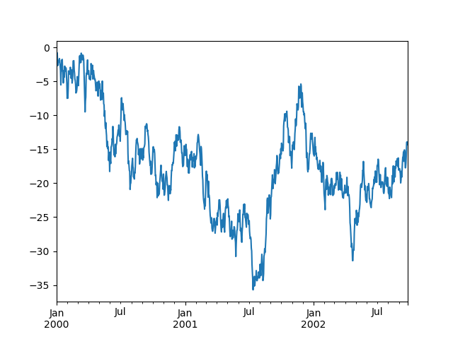
WARNING
在Jupyter中,使用plot()时绘图将会出现。否则,使用matplotlib.pyplot.show来显示它,或使用matplotlib.pyplot.savefig将其写入文件。
plot()绘制所有列:
In [129]: df = pd.DataFrame(
   .....:     np.random.randn(1000, 4), index=ts.index, columns=["A", "B", "C", "D"]
   .....: )
   .....:

In [130]: df = df.cumsum()

In [131]: plt.figure();

In [132]: df.plot();

In [133]: plt.legend(loc='best');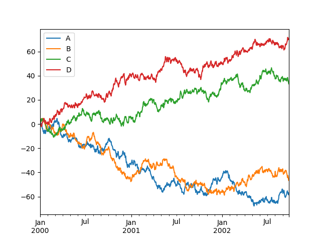
导入和导出数据
请参阅IO工具部分。
CSV
In [134]: df = pd.DataFrame(np.random.randint(0, 5, (10, 5)))

In [135]: df.to_csv("foo.csv")In [136]: pd.read_csv("foo.csv")
Out[136]:
Unnamed: 0 0 1 2 3 4
0 0 4 3 1 1 2
1 1 1 0 2 3 2
2 2 1 4 2 1 2
3 3 0 4 0 2 2
4 4 4 2 2 3 4
5 5 4 0 4 3 1
6 6 2 1 2 0 3
7 7 4 0 4 4 4
8 8 4 4 1 0 1
9 9 0 4 3 0 3Parquet
写入Parquet文件:
In [137]: df.to_parquet("foo.parquet")从Parquet文件存储中读取,使用read_parquet():
In [138]: pd.read_parquet("foo.parquet")
Out[138]:
   0  1  2  3  4
0  4  3  1  1  2
1  1  0  2  3  2
2  1  4  2  1  2
3  0  4  0  2  2
4  4  2  2  3  4
5  4  0  4  3  1
6  2  1  2  0  3
7  4  0  4  4  4
8  4  4  1  0  1
9 0 4 3 0 3Excel
读写Excel。
使用DataFrame.to_excel()写入excel文件:
In [139]: df.to_excel("foo.xlsx", sheet_name="Sheet1")使用read_excel()从excel文件读取:
In [140]: pd.read_excel("foo.xlsx", "Sheet1", index_col=None, na_values=["NA"])
Out[140]:
   Unnamed: 0  0  1  2  3  4
0           0  4  3  1  1  2
1           1  1  0  2  3  2
2           2  1  4  2  1  2
3           3  0  4  0  2  2
4           4  4  2  2  3  4
5           5  4  0  4  3  1
6           6  2  1  2  0  3
7           7  4  0  4  4  4
8           8  4  4  1  0  1
9 9 0 4 3 0 3注意事项
如果你试图在Series或DataFrame上执行布尔运算,你可能会看到类似以下的异常:
In [141]: if pd.Series([False, True, False]):
   .....:      print("I was true")
   .....:
---------------------------------------------------------------------------
ValueError                                Traceback (most recent call last)
<ipython-input-141-b27eb9c1dfc0> in <module>()
----> 1 if pd.Series([False, True, False]):
      2      print("I was true")

~/work/pandas/pandas/pandas/core/generic.py in __nonzero__(self)
   1578     @final
   1579     def __nonzero__(self) -> NoReturn:
-> 1580         raise ValueError(
   1581             f"The truth value of a {type(self).__name__} is ambiguous. "
   1582             "Use a.empty, a.bool(), a.item(), a.any() or a.all()."
   1583         )

ValueError: The truth value of a Series is ambiguous. Use a.empty, a.bool(), a.item(), a.any() or a.all().